Adversarial Tutorial
ARLIN can be used from an adversarial standpoint to identify the optimal timing for attacks against a policy. Most adversarial methods focus on attacking at a given frequency, or by measuring internal metrics from the model and choose actions based on which actions are seen as “the worst” by the model.
Using ARLIN, we can identify clusters that represent mission failure and use the SAMDP to analyze which clusters we should attack in and which actions to take to ensure the policy ends in a failure. Since the SAMDP maps actions that the agent has actually taken in the XRLDataset, the resulting attacks will not only be effective, but also less noticeable to an observer as the attack will look more natural and similar to how the policy would truly react in the scenario.
Below is a simple example of ARLIN being used for adversarial attack enhancement.
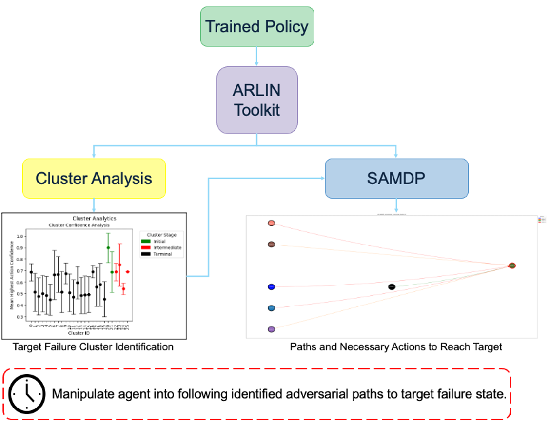 Figure 1. Example workflow of how ARLIN can be used for adversarial purposes.
Note: We use the analysis from the explainability tutorial as a basis for our attacks. We recommend reading that tutorial before this one.
To give examples of traditional adversarial attacks and a baseline performance of the policy, we show gifs from a variety of methods. We can see that all adversarial methods result in very noticeable failures that are very different from the path the policy would normally take. ARLIN aims to time an attack so that it is less noticeable than the below, but still effective.

Figure 2. Gifs created from baseline performance and traditional adversarial attacks. Baseline is the policy with no attacks, Worst1 is the worst possible action at every step , Worst10 is the worst possible action at every 10 steps, and Pref75 takes the worst possible action when the delta between the probabilities of the most and least probable action is above a threshold of .75 (left to right: Baseline, Worst1, Worst10, Pref75).
from arlin.samdp import SAMDP

samdp.save_terminal_paths('./paths_into_23.png`,
                            best_path=True,
                            term_cluster_id=23)
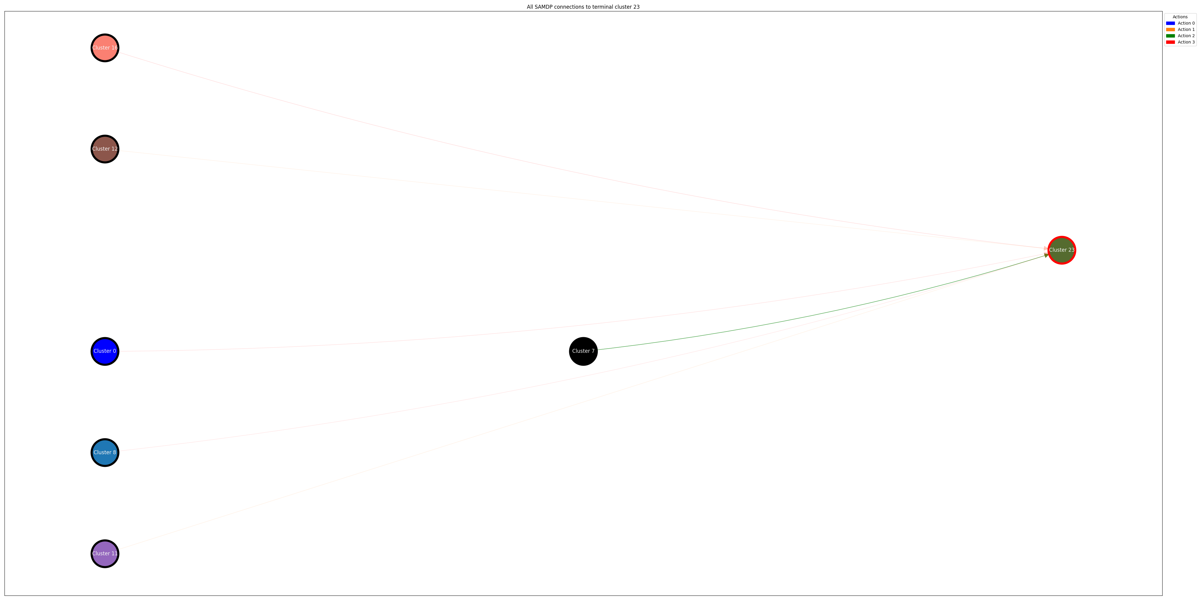 Figure 3. Neighboring clusters and associated actions for moving into Cluster 23.
Figure 3 shows us the clusters that are connected to our target cluster, Cluster 23, along with the actions that are most likely to result in the agent moving into our target cluster. We can use this from an adversarial perspective to manipulate the agent into moving into our target cluster, resulting in mission failure.
By using ARLIN to analyze the policy, we identify the potential paths to Cluster 23 as taking action 2 when in Cluster 7, action 3 when in Clusters 16, 0, and 8, and action 1 when in Clusters 11 and 12. During the course of the episode, we monitor the current cluster of the agent. Once the agent reaches one of the identified clusters, we influence the agent to take the specified action. This results in an attack that follows the policy for majority of the episode, and only attacks when it results in a failure that is normal for the policy to find (Figure 3). In trials, this approach results in the agent reaching the target cluster 90% of the time.
Figure 4. ARLIN influenced attack, showing how the attack results in a reasonable failure as opposed to an obvious one as seen in Figure 1.
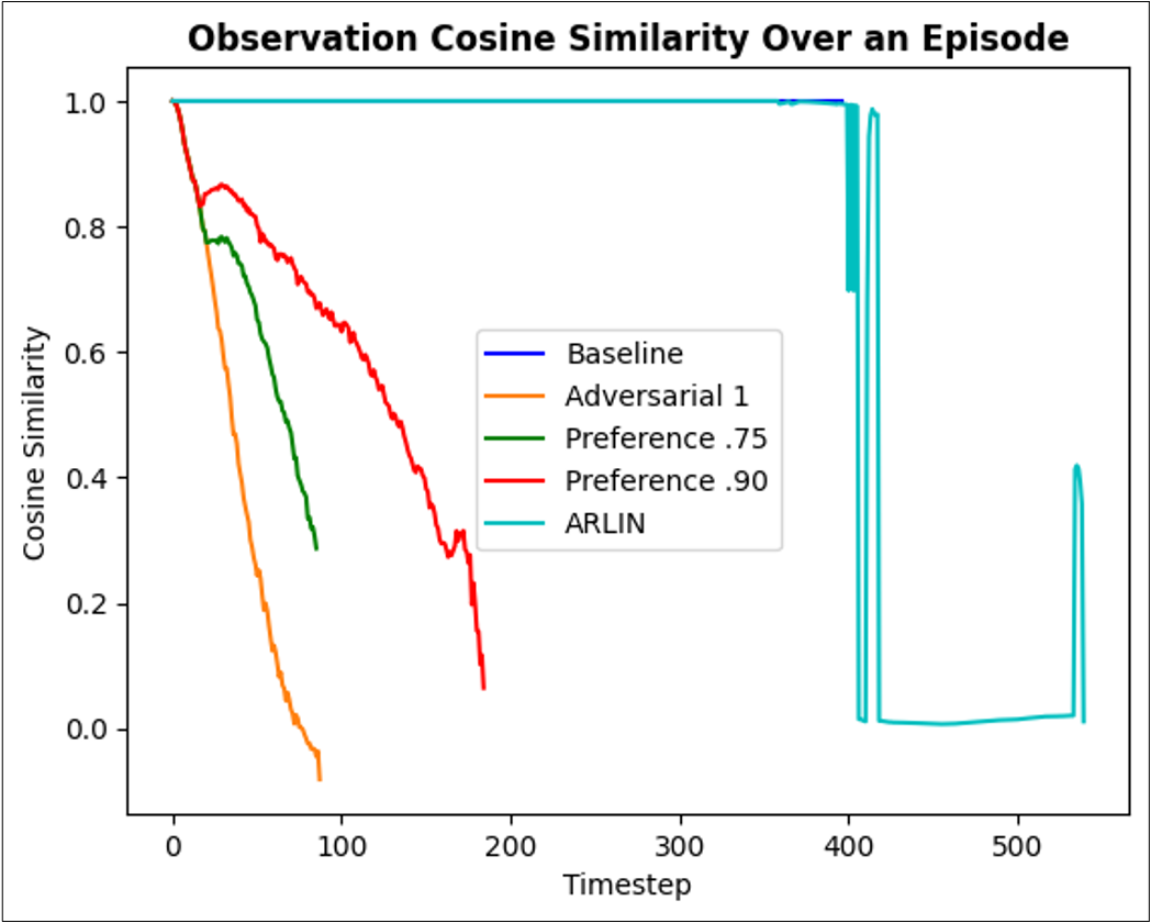
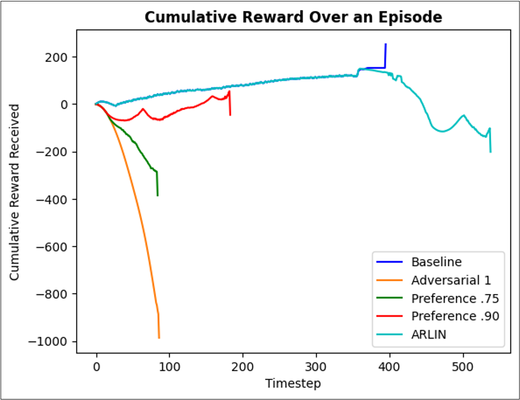
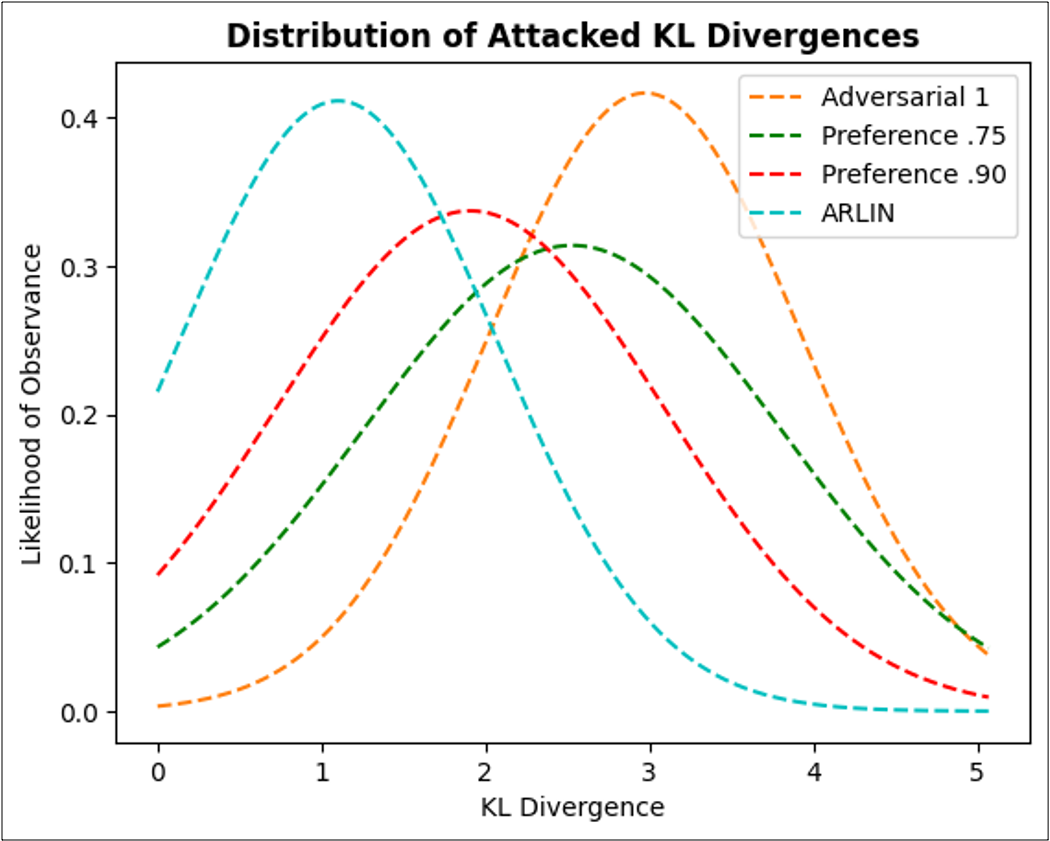
Figure 5. Detectability metrics illustrating ARLIN's usage in adversarial attack timing. Left to right: cosine similarity over an episode, cumulative reward over an episode (same episode as cosine similarity), average kl_divergence distribution over 25 episodes.
In Figure 5, attacked plots for cosine similarity and cumulative reward that closely resemble the baseline (non-attacked) plot are considered less detectable attacks to an observer. As the attacked plot strays from the non-attacked plot, the attack will become more visible as it is very out of the norm. Attacks that closely follow the path of the non-attacked agent except at limited points will look more like an error than an attack. In both figures, ARLIN follows the non-attacked policy for most of the episode, and only strays once the target clusters are reached, resulting in a quick movement to the target failure state and a reduction in overall reward received.
In the KL Divergence graph in Figure 5, distributions that are closer to 0 are less detectable to an observer. If the action distribution of an attacked policy is similar to the distribution of the non-attacked policy, then the adversarial action is seen as a “reasonable” action by the policy. ARLIN’s distribution is the closest to 0 out of all methods, meaning the adversarial actions identified by ARLIN are more “reasonable” and therefore less detectable.